Setup
Two things before we start:
- How this book is put together, and
- What to install.
The first part takes two minutes to read and will make the rest of the course easier to follow.
How this book works
The book is longer than the course
The course is six hours. The book has more in it than six hours can cover, and that is on purpose.
We follow one path through it live, and the rest stays here for when you want it. So if we skip a section, or if you notice a box we never opened, nothing has gone wrong - it is there for you to come back to. I would rather write the complete version and choose what to teach on the day than write only what fits and leave you with notes that stop where the session did.
How we will work
Mostly by typing. I will write code, you write it too, and we will break things together and then fix them. You will get more out of this by typing the examples than by watching me type them, even when it feels slower.
You do not need to keep up with every keystroke. Everything on screen is in the book, with a copy button on every code block.
The boxes
Four kinds of box turn up throughout, each with its own colour and icon:
- ✏️ Your Turn - something for you to do. Most of these we do together in the session, and a few are there for afterwards. The ones that ask what you think have no wrong answers; I am genuinely curious what has gone wrong for you before.
- 🕰️ Some history - where something came from. Why a linter is called a linter, where the backslash in
\(x)comes from. Entirely skippable, and quietly my favourite part of the book. - 🔎 Going deeper - optional extra detail, a longer example, or a list you might want later. Boxes titled Read more point at the blog post or talk a section is adapted from, so you can follow the original if you want it.
- 🚨 - the things that will actually bite you. There are not many, and that is deliberate.
Rather than describe them, here is one of each.
Exercises look like this. Most of them give you something to run:
Some of them just ask you something. Here is the one I actually care about: what is the worst R code you have ever had to work with? Your own counts, and mine definitely does.
There is no wrong answer. I am asking because the answer usually tells me which parts of the day to slow down on.
Two things at once, which I think is lovely.
R was written by Ross Ihaka and Robert Gentleman at the University of Auckland in the early 1990s, and they share a first initial. It is also a play on S, the language it was modelled on, in the same way that C came after B.
So the name is a pun and a signature at the same time. You can read their own account of it in R: A Language for Data Analysis and Graphics.
You just clicked a title, so that is the collapsing demonstrated.
These are Quarto callouts, and there is nothing clever going on. Each one is a fenced div with a class on it:
The colours and the icons come from a stylesheet in the book’s repo, not from Quarto. Quarto ships five callout types with its own icons, and I have repainted all five.
If you want them in your own work, the docs are at Quarto: callout blocks.
If you install a package that is already loaded in your session, R can end up half on the old version and half on the new one. You then get errors that make no sense and do not survive a restart, which is a miserable way to spend twenty minutes.
So once you have worked through the installs below, restart R. In RStudio that is Cmd / Ctrl + Shift + F10.
Some boxes are collapsed, showing only their title, like the Going deeper one above. Click the title to open one. If you are reading the PDF they are all open already, which is one reason the PDF is longer than it looks online.
The code
Code blocks look like this:
Lines starting with #> are output, not code. You do not type those - they are what R prints back, shown so you can check you got the same thing.
Longer blocks have line numbers in the margin so that I can say “look at line 4” and we are both looking at the same line. Short blocks do not, because there is nothing to point at.
Most examples use data that comes with R, like airquality above, so you can run anything here without downloading a dataset first.
We use the base pipe, |>, rather than %>% throughout. If you are used to %>%, everything here works the same way.
Where everything lives
- This book - https://r-best-practices.njtierney.com, and there is a PDF download in the sidebar if you would rather print it or annotate it.
- The book’s source - https://github.com/njtierney/rbestpractices. Every page has an “Edit this page” link, which goes straight to the file that made it.
- The books exercises - https://github.com/njtierney/rbp-exercises. We will discuss how to “automagically” open this in the course
If you find a mistake, please tell me. Every page has a link to open an issue, or you can email me. Errors in teaching material are worth more than errors in almost anything else I write, because thirty people hit them at once. Finding one is a favour, not a complaint.
What to install
If you can, it is worthwhile to install the below before the first session.
We have time on the day, and I would much rather spend ten minutes helping you get set up than have you sit out an exercise. So work through what you can, and bring the rest along.
R
You need R 4.5.0 or later, from https://cran.r-project.org/. Check what you have with:
The reason for 4.5.0 specifically is the penguins. From that version, R ships a penguins dataset with base R, so a few of the examples work without installing anything at all. Before 4.5.0, you had to get it from a package.
You also need an editor - the thing you use to edit your R code.
Personally, I recommend RStudio.
If you like, you can use Positron - for this course I mostly focus on RStudio, but am able to discuss some of the features with positron, which is posit(the company that made RStudio)’s latest generation tool.
If you already have one and you like it, stay where you are.
Everything in the course still works, but you will need the palmerpenguins package for the handful of examples that use penguins:
One catch: the column names are different. When the data moved into base R the names were shortened, so you will need to translate:
| In this book | In palmerpenguins |
|---|---|
bill_len |
bill_length_mm |
bill_dep |
bill_depth_mm |
flipper_len |
flipper_length_mm |
body_mass |
body_mass_g |
The units left the names but not the data - body_mass is still in grams.
I wrote about this and the rest of what landed in 4.5.0 here: R version 4.5.0 is out.
You can use Ella Kaye’s basepenguins R package to help you move your existing scripts across if you want to use base R penguins.
Separately, some examples read a penguins.csv file rather than the dataset. Those use the longer names, because that is what is in the file - not because of your R version.
The R packages
It might will take a few minutes:
sf and sp are only needed for one optional exercises. They are the heaviest things on the list, so if they give you trouble, leave them and let me know.
Code formatters
Air is an R formatter from Posit. It is not an R package, so it installs from the terminal rather than from R.
See their installation instruction on their website:
But briefly, here are the most popular ways to install:
On macOS and Linux:
On Windows:
Check it worked:
You should get a version number back. If you get “command not found”, the install did not finish, so try it again.
We set up format-on-save together in chapter 2, so there is nothing else to do with air before we start.
If you have trouble installing {air}, {styler} is in the package list above and does the same job, just not as fast.
Jarl, the linter
Jarl is a fast linter by Etienne Bacher, built on top of Air. Installation instructions are on its site.
Jarl is optional. Like air, it is a command line tool rather than an R package, so the install can go wrong in all the same ways, and I do not want you fighting it before we start.
If it gives you any trouble, do not worry about it. {flir} is in the package list above - it is by Etienne as well, it installs the way every other R package installs, and it is the one that will still fix things for you. {lintr} is in the list too. Everything in chapter 2 works with any of the three.
Checking it all worked
Run this in R. It should print TRUE for everything.
Then, in the terminal:
If both of those look right, you are set.
If something will not install
Please do send me an email before the session rather than fighting with it on your own.
Installation problems are almost always specific to one machine, and they are much faster to solve with two people looking at them. They are also, genuinely, not a reflection on you. Every one of us has lost an afternoon to a package that would not build. Ask me for some horror stories.
Get course exercise materials on your machine
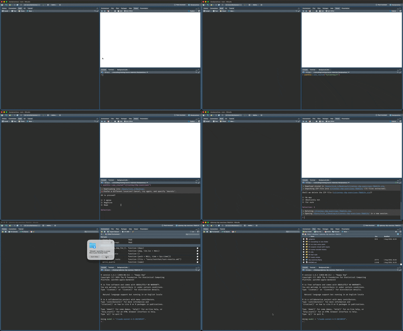
Let’s download the course exercise - try running this code:
Which will prompt you to download the repository, https://github.com/njtierney/rbp-exercises, and then open it in an RStudio project.
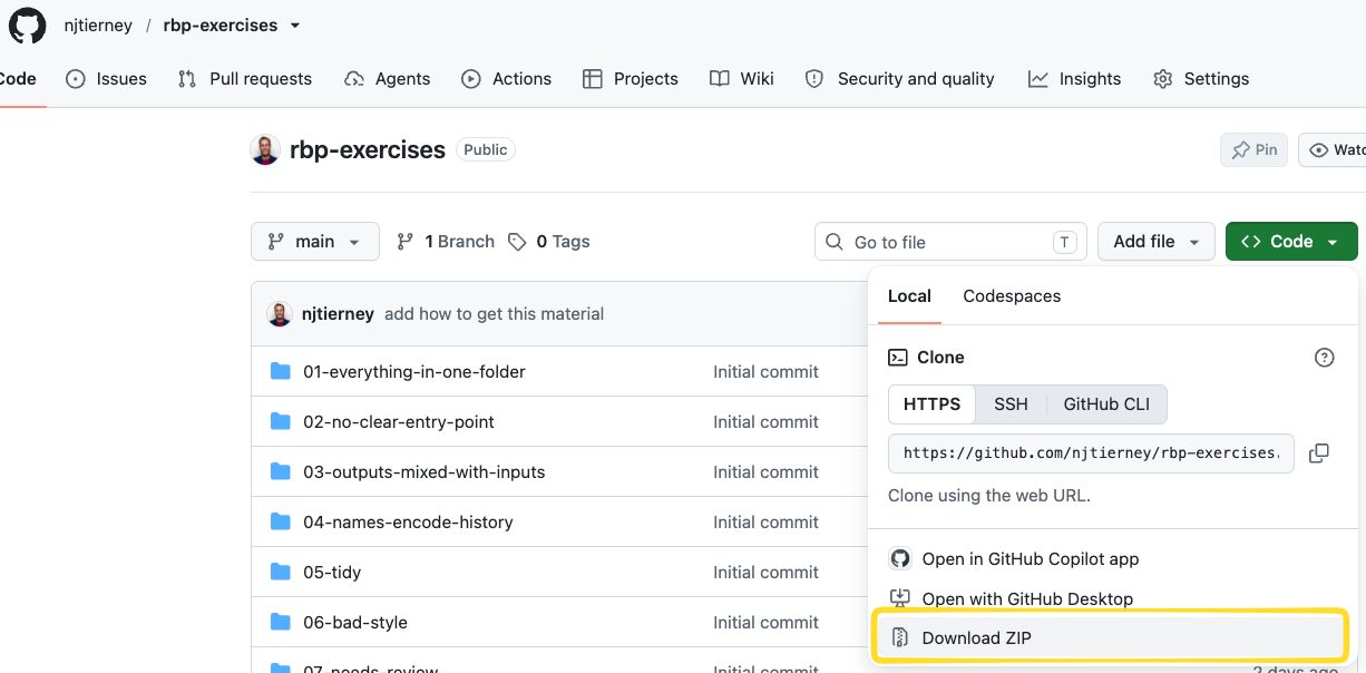
If you have troubles with this (sometimes firewalls can stop you) you can download it from the github page https://github.com/njtierney/rbp-exercises like so:
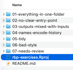
Then, unzip that, and click on the rbp-exercises.Rproj file:
Links
- R: A Language for Data Analysis and Graphics
- Quarto: callout blocks
- https://r-best-practices.njtierney.com
- https://github.com/njtierney/rbestpractices
- https://github.com/njtierney/rbp-exercises
- https://cran.r-project.org/
- RStudio
- Positron
- palmerpenguins
- R version 4.5.0 is out
basepenguins- Air
- Jarl
- Etienne Bacher